
How MRI Image Reconstruction Methods Turn Scan Data Into Images
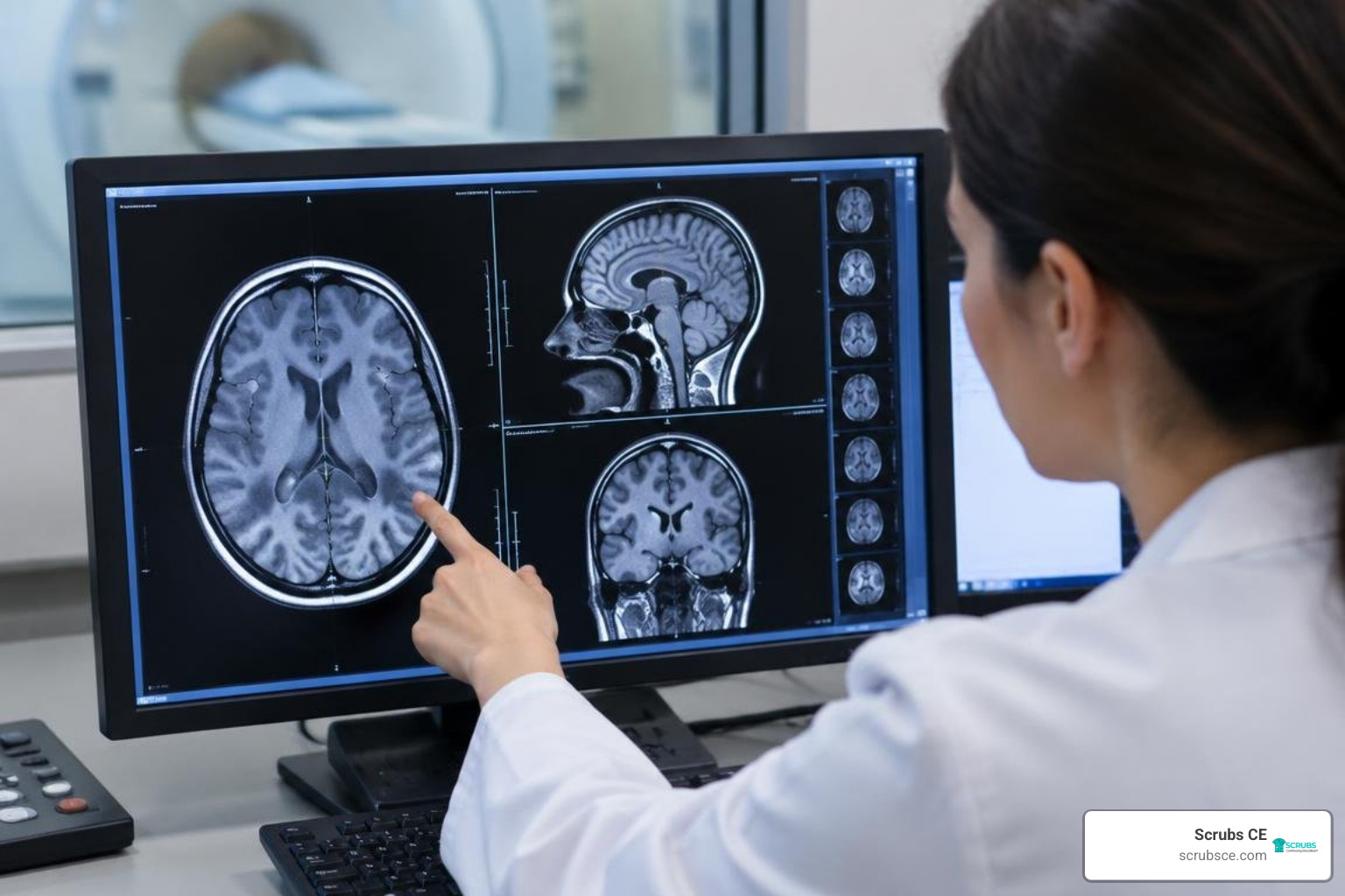
MRI image reconstruction methods turn raw scanner data, called k-space data, into images. A standard scan can use a Fourier transform to make an image. Faster scans collect less data, so they need methods to fill in what is missing: parallel imaging uses signals from multiple coils, compressed sensing uses patterns in the image, and newer deep learning methods learn from examples. The goal is to shorten scan time without losing details that matter for diagnosis.
These methods differ in how they handle missing data, how much computing they need, and how well they work across scan types. This guide explains those trade-offs, from established techniques to physics-guided neural networks.
I am Zita Ewert, a continuing education leader at Scrubs CE who helps imaging professionals stay current with changing technology and practice requirements. My work includes making topics such as mri image reconstruction methods easier to learn alongside ARRT® (AMERICAN REGISTRY OF RADIOLOGIC TECHNOLOGISTS®) requirements.
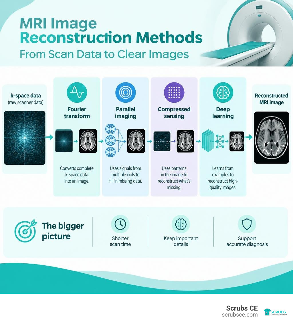
Mri image reconstruction methods terms to know:
Foundations of the Inverse Problem and Classical Reconstruction
Magnetic resonance imaging is one of the most versatile diagnostic tools in clinical medicine, with over 100 million scans performed worldwide each year. Yet, every scan faces a core physical challenge: we cannot photograph the human body’s interior directly. Instead, receiver coils capture raw spatial-frequency signals in the Fourier domain, known as k-space. Transforming these frequency samples back into an interpretable spatial image constitutes an ill-posed mathematical inverse problem.
In a fully sampled acquisition, the physical encoding process obeys the Nyquist-Shannon sampling theorem. Applying a standard 2D inverse Fast Fourier Transform (FFT) yields a sharp anatomical image. The linear forward model is expressed as:
$$y = A x + \epsilon$$
Here, $y$ represents the acquired multi-channel k-space measurements, $x$ is the true underlying complex-valued anatomical image, $A$ is the forward encoding operator incorporating spatial phase encoding, Fourier transformation, and receiver coil sensitivity profiles, and $\epsilon$ represents thermal and electronic noise.
When clinical teams accelerate scan times to enhance patient comfort or limit motion artifacts, technologists skip lines along the phase-encoding direction. This k-space undersampling violates the Nyquist limit, introducing severe wrap-around aliasing and coherent ghosting across the reconstructed field of view. To resolve these ambiguities, classical reconstruction techniques rely on spatial information from multi-channel receiver arrays or mathematical regularization priors. Mastering these foundational mechanisms begins with essential foundational MRI training.
Parallel imaging (PI) methods were the earliest clinical standard for sub-Nyquist reconstruction:
- SENSE (Sensitivity Encoding): Solves linear systems in the image domain by utilizing spatial sensitivity maps calculated across receiver coil arrays.
- GRAPPA (GeneRalized Autocalibrating Partially Parallel Acquisitions): Operates directly in k-space, synthesizing missing phase-encoding lines via localized convolutional weight kernels derived from fully sampled auto-calibration signal (ACS) lines.
When noise amplification or high acceleration factors make direct unaliasing unstable, algorithms incorporate Tikhonov regularization ($\lambda^2 I$) to penalize excessive energy and condition the underlying inversion matrices, as detailed in direct pseudoinverse reconstruction research.
Direct Inversion and Algebraic Solvers
For decades, direct matrix pseudoinverse reconstruction (Pinv-Recon) was considered computationally intractable for everyday clinical scanners because direct pseudoinversion has an algebraic complexity of $\mathcal{O}(N^3)$. Storing a dense system matrix for a modest $128 \times 128$ image grid can consume over 2 GB of memory, which overwhelmed older 32-bit hardware.
Modern multi-threaded processors and high-memory GPUs have revived algebraic direct solvers. Rather than computing full Singular Value Decomposition (SVD), modern pipelines solve regularized normal equations through the Gram matrix:
$$(A^H A + \lambda^2 I) x = A^H y$$
Applying Cholesky factorization to this Hermitian positive-definite system delivers a ~100x speedup over standard SVD. Furthermore, running these dense matrix factorizations on modern GPUs yields speedups between 1.7x and 7.8x for systems larger than 2 GB compared to multi-threaded CPUs.
Direct algebraic reconstruction offers distinct advantages:
- Analytical Transparency: It enables direct calculation of the Spatial Response Function ($SRF = \text{Recon} \times A$), quantifying exact point-spread blurring and inter-voxel crosstalk.
- Explicit Noise Tracking: Technologists and researchers can calculate the exact noise covariance propagation matrix across the field of view.
- Trajectory Flexibility: Non-Cartesian acquisitions (such as spiral and radial trajectories) and off-resonance field map corrections ($B_0$) can be folded into the forward operator $A$ without iterative convergence loops.
Compressed Sensing and Hand-Crafted Priors
When acceleration factors exceed the spatial encoding capability of receiver coil arrays (e.g., $R \ge 3$), Parallel Imaging alone suffers from elevated noise amplification (quantified by high $g$-factor penalties). Compressed Sensing (CS-MRI) overcame this barrier by exploiting transform sparsity.
CS-MRI operates on three core principles:
- Transform Sparsity: Diagnostic MR images exhibit sparse representations in mathematical transform domains, such as discrete wavelets, curvelets, or spatial finite differences (Total Variation, TV).
- Incoherent Aliasing: Undersampling k-space pseudo-randomly or along non-Cartesian trajectories spreads aliasing energy into diffuse, noise-like interference rather than sharp coherent ghosts.
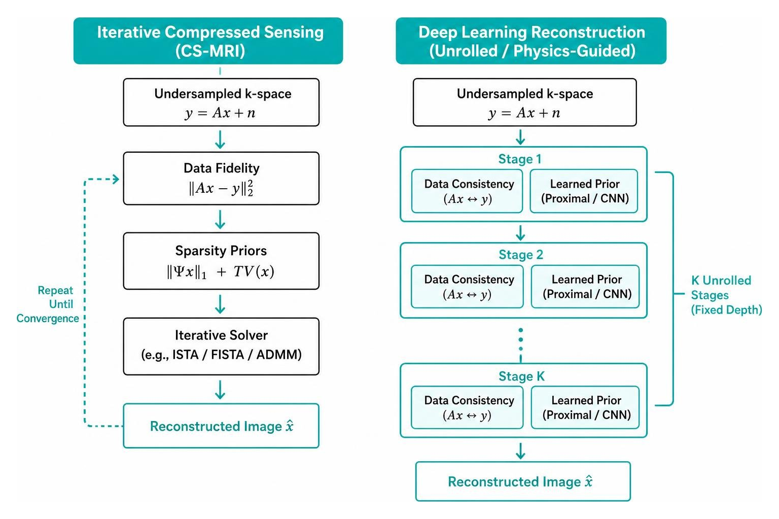
- Non-Linear Iterative Solvers: An unconstrained objective function balances data fidelity with prior sparsity penalties:
$$\min_{x} \frac{1}{2} \| A x – y \|2^2 + \lambda1 \| \Psi x \|1 + \lambda2 \text{TV}(x)$$
Where $\Psi$ is a sparsifying transform operator and $\lambda$ controls regularization strength. For clinicians looking to connect physical k-space filling with clinical sequence parameters, exploring applied clinical imaging physics provides invaluable practical context.
Despite cutting scan times by up to 80%, classical CS has inherent operational limitations. Hand-crafted priors treat complex anatomical variations uniformly, which can wash out subtle structural boundaries or produce “staircasing” artifacts at aggressive acceleration factors.
Physics-Guided and Unrolled MRI Image Reconstruction Methods
While early deep learning implementations deployed black-box convolutional networks (such as U-Nets) to denoise zero-filled images, they frequently struggled with hallucinated anatomical structures or discarded true underlying lesions. To guarantee physical validity, modern clinical methods use physics-guided unrolled neural networks.
Unrolled architectures map classical iterative optimization algorithms—such as Proximal Gradient Descent, the Alternating Direction Method of Multipliers (ADMM), or Primal-Dual Hybrid Gradients—into a fixed number of cascaded network stages. Each unrolled stage alternates between two operations:
- Learned Regularization Block: A convolutional or attention network acts as an implicit proximal operator, removing artifacts and restoring image features.
- Physical Data Consistency (DC) Layer: A non-trainable layer enforces fidelity with actual scanner measurements by replacing predicted k-space lines with real acquired data points ($y$):
$$x^{(k+1)} = \arg\min_x \frac{1}{2} \| A x – y \|_2^2 + \frac{\mu}{2} \| x – z^{(k)} \|_2^2$$
Where $z^{(k)}$ is the denoised output from the network block at iteration $k$.
By unrolling Maximum a Posteriori (MAP) estimation into an end-to-end differentiable computational graph, these architectures retain physical interpretability while allowing backpropagation to optimize regularizer weights across large training cohorts.
Unrolled Gradient Architectures and DDGU-Net
A major challenge in high-acceleration unrolled networks is the progressive loss of high-frequency anatomical boundaries. Standard MSE loss functions over-penalize sharp gradient outliers, creating smooth but blurred tissue interfaces.
Recent advancements in gradient-enhanced unrolling research demonstrate that integrating explicit gradient priors directly into unrolled architectures resolves this limitation. The Deep Deviation Gradient Unrolling Network (DDGU-Net) pairs deep priors with a Cumulative Deviation from Maximum Gradient magnitude (CDMG) prior.
DDGU-Net incorporates multi-order gradient operators into its likelihood terms to guide image reconstruction:
- CDMG Statistical Modeling: Explicitly models the distribution of maximum gradient magnitudes extracted from fully sampled reference images, establishing physical constraints on edge sharpness.
- Multi-Order Likelihood Formulation: Incorporates first- and second-order spatial derivatives into data consistency updates, ensuring that fine trabecular and cortical bone structures are recovered.
- Balanced MAP Unrolling: Balances explicit physically grounded constraints with data-driven neural priors, delivering state-of-the-art detail retention on benchmarks like fastMRI.
Plug-and-Play Optimization and Convergence Guarantees
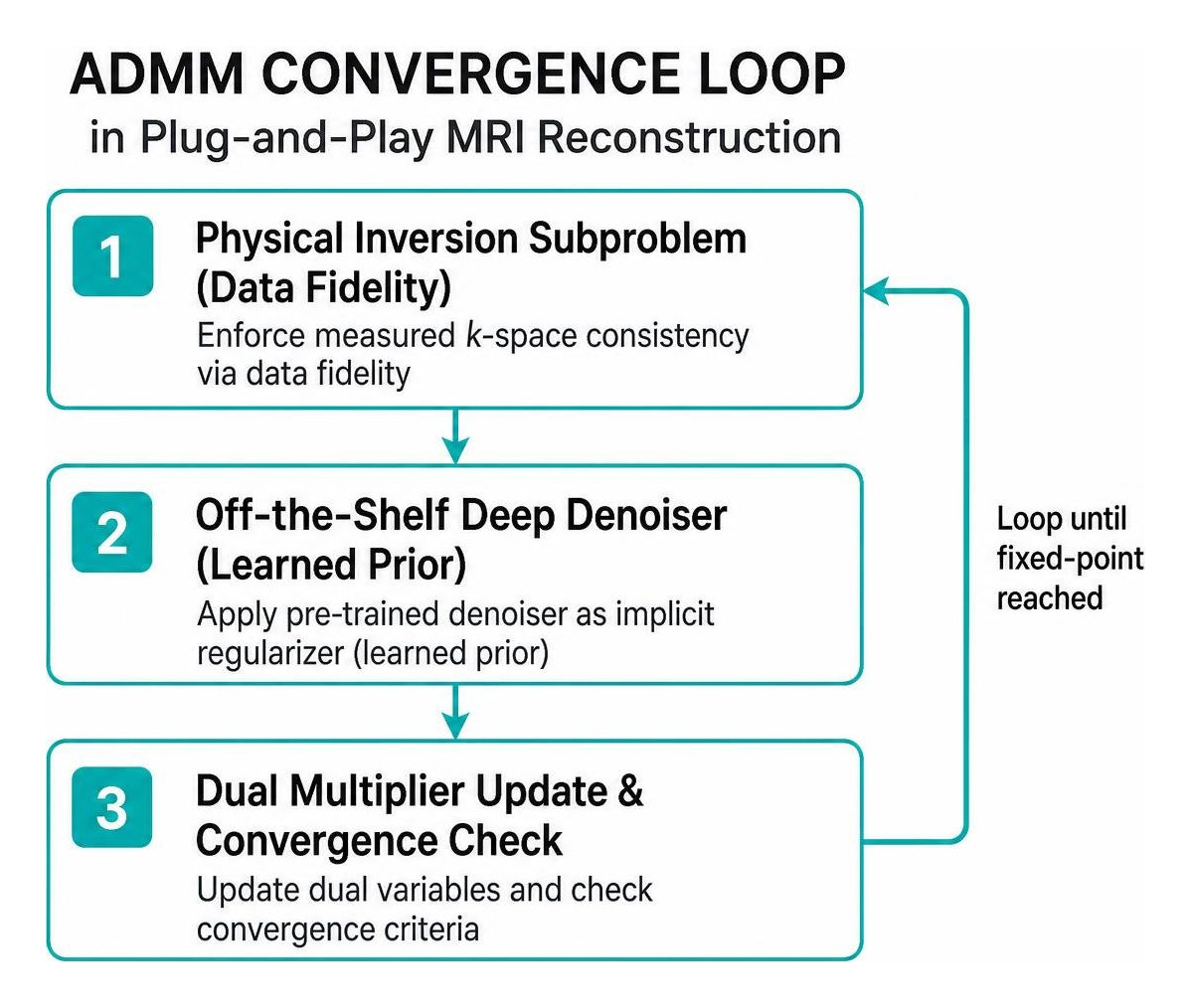
Plug-and-Play (PnP) frameworks offer an alternative modular paradigm. Rather than training an end-to-end unrolled network for a specific acceleration factor, PnP methods embed pre-trained, standalone denoisers into classical optimization loops (such as ADMM or Douglas-Rachford splitting).
A common concern with standard PnP algorithms has been theoretical stability—iterative loops running non-linear deep denoisers can diverge or settle into unphysical artifacts.
The PALADIN 3D CS-MRI architecture addresses this challenge for volumetric imaging by combining two complementary regularizers:
- Tensor Tubal Nuclear Norm (TNN): Exploits global low-rank redundancies across all three spatial dimensions, preserving continuous 3D anatomy.
- Dual Implicit Deep Regularizers: Pairs a learned 3D CNN denoiser with a dedicated deep CS-MRI optimizer within an ADMM framework.
- Fixed-Point Convergence Proof: Extends operator-splitting theory to guarantee mathematical convergence to a stationary fixed point under bounded Lipschitz conditions, protecting against erratic reconstruction behavior.
Implicit Neural Representations and Transformer Architectures
Beyond standard discrete pixel grids, modern reconstruction methods explore continuous coordinate mappings and attention mechanisms. These approaches help eliminate grid-discretization errors and improve scalability across various scan parameters.
Implicit Neural Representations (INRs) reframe image reconstruction from estimating discrete pixel arrays to learning continuous coordinate functions:
$$f_\theta: (u, v, w) \mapsto (\text{Magnitude}, \text{Phase})$$
By feeding spatial coordinates $(u, v, w)$ through high-frequency Fourier positional encodings into a multi-layer perceptron (MLP), INRs model images as continuous volumetric fields. This framework allows practitioners to query arbitrary spatial locations and synthesizes fine structures without fixed resolution boundaries. Understanding these smart scanning architectures is increasingly central to evaluating advances in modern scanner intelligence.
Generalized INR for Arbitrary Undersampling Scales
Early INR frameworks suffered from a notable clinical drawback: they were scan-specific, requiring test-time optimization that took anywhere from 20 minutes to over 4 hours per patient.
Modern generalized implicit neural representation studies eliminate this bottleneck through scale-embedded encoders. Rather than optimizing network weights from scratch for every scan, a generalized INR trains once on population data, extracting scale-independent latent tokens that modulate downstream coordinate decoders.
Key performance metrics demonstrate the operational advantages of generalized INR systems:
- Compute Efficiency: Decreases GPU memory utilization to 62.8% and cuts training and inference runtimes to 19.6% compared to transformer baselines.
- Inference Speed: Reconstructs 50 image slices in 2.80 seconds (compared to 0.33 to 4.53 hours for scan-specific INRs) and 500 volumetric slices in 28.07 seconds (versus 3.09 to 46.24 hours).
- Scale Agility: Generalizes across multiple acceleration factors ($4\times, 5\times, 6\times$) within a single model instance without retraining.
- Quantitative Quality: Achieves an SSIM of 0.9761 and PSNR of 43.23 dB on fastMRI brain data at $4\times$, and an SSIM of 0.9729 with PSNR of 43.13 dB on knee data at $6\times$.
- Direct k-Space Rendering: Predicts complex phase angles alongside real magnitude, matching physical receiver signals in k-space.
Cascaded Vision Transformers and Swinμ Blocks
Vision Transformers (ViTs) provide wide receptive fields that capture long-range contextual correlations across structural tissues. However, full self-attention scales quadratically ($\mathcal{O}(N^2)$), causing substantial memory overhead when processing multi-coil raw arrays.
To address this challenge, cascaded Swin transformer research introduced cascaded architectures built with compact Swinμ micro-blocks and shifted, overlapped window attention.
Architectural innovations within the Swinμ framework include:
- Overlapped Window Attention: Implements a ~50% spatial overlap between adjacent attention windows, extending the model’s receptive field across window boundaries without quadratic memory expansion.
- Swinμ Micro-Blocks: Reduces sub-block depth to three layers, enabling deeper cascades (up to 13 stages) within standard 24 GB to 48 GB GPU hardware budgets.
- Parameter Efficiency: Decreases parameter counts from 20.8M down to 5.5M–11.9M while outperforming heavy baseline CNN models on both high-field (3.0T) and low-field (0.3T) clinical datasets.
Quantitative Benchmarks, Translation, and Clinical Validation
Evaluating mri image reconstruction methods requires robust quantitative validation against standardized benchmarks, followed by qualitative review from board-certified radiologists.
Standard benchmark datasets include:
- fastMRI (NYU Langone Health & Meta AI): Over 1,500 fully sampled knee and brain diagnostic datasets.
- Calgary-Campinas (University of Calgary): Multi-channel raw clinical brain acquisitions across various field strengths.
- M4Raw: Multi-contrast low-field brain imaging datasets.
As outlined in this comprehensive tutorial on clinical MRI reconstruction, selecting an architecture involves balancing visual quality, reconstruction speed, and hardware costs.
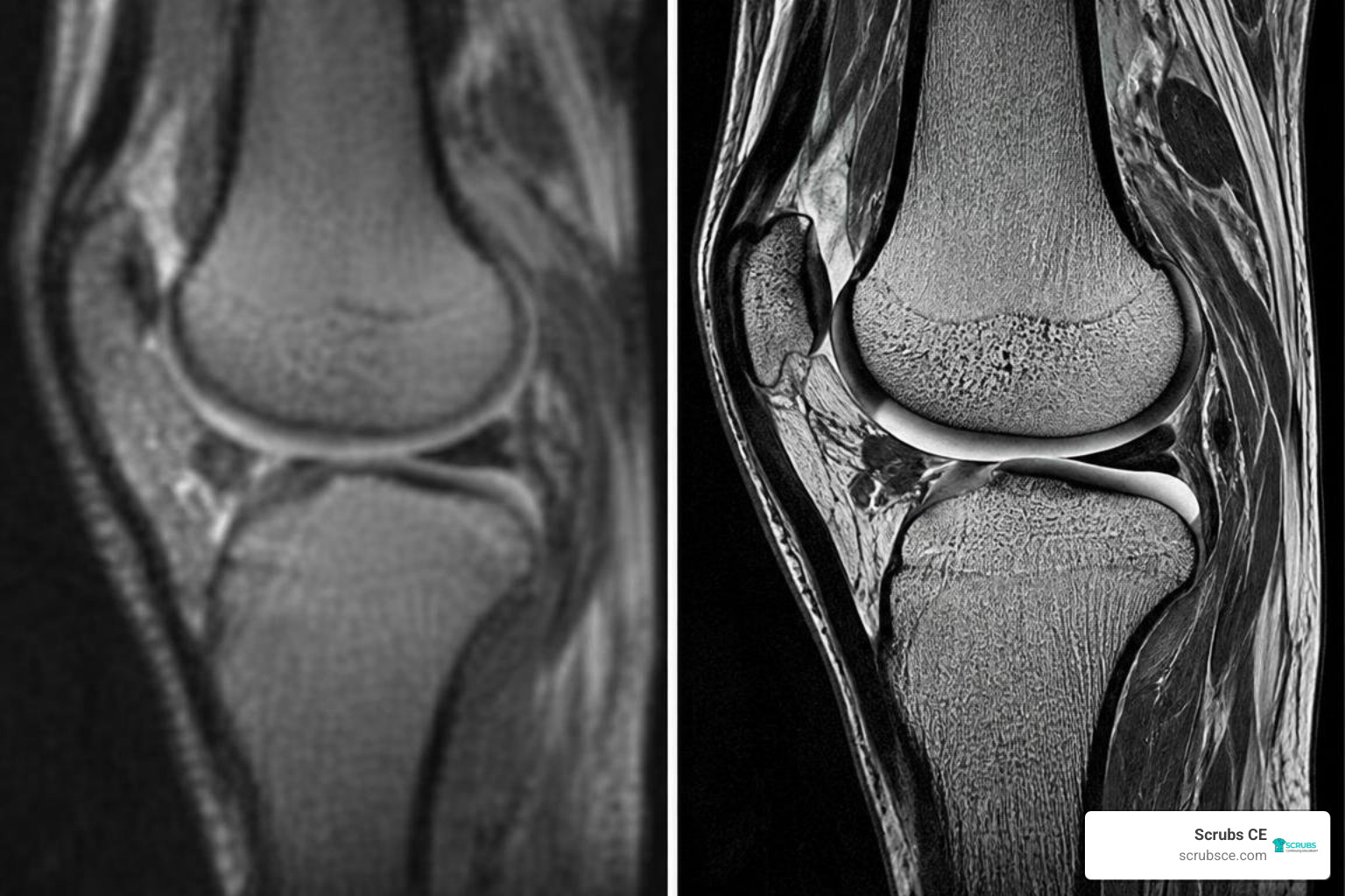
Evaluating Modern MRI Image Reconstruction Methods
Moving deep learning reconstruction models from research labs into clinical Radiology suites requires addressing several practical challenges:
- Suppression of Hallucinations: Purely generative networks can occasionally produce plausible-looking structural patterns that do not reflect true anatomy. Physics-based data-consistency layers mitigate this risk by tethering outputs directly to the acquired raw k-space data.
- Pathology Generalization: Models trained primarily on healthy volunteers must be evaluated on rare clinical conditions, such as microbleeds, torn ligaments, and infiltrating neoplasms, to ensure diagnostic sensitivity is maintained.
- Hardware Integration: Modern clinical scanners must reconstruct multi-slice imaging volumes within seconds to prevent PACS workflow bottlenecks.
- Radiologist Reader Studies: Quantitative improvements in PSNR and SSIM must translate to equal or superior diagnostic accuracy, lesion conspicuity, and artifact scores during blinded radiologist reviews.
Emerging Frontiers in MRI Image Reconstruction Methods
Reconstruction research continues to expand across several innovative fronts:
- Self-Supervised & Unsupervised Learning: Novel training frameworks train networks using only undersampled k-space measurements, bypassing the need for fully sampled ground-truth acquisitions.
- Multi-Contrast Synergy: Cross-attention transformer blocks leverage structural redundancies across co-acquired sequences (such as T1, T2, and FLAIR) to accelerate total exam protocols.
- Low-Field Point-of-Care Imaging: Tailored neural architectures reduce noise and correct for non-uniform magnetic fields on accessible 0.05T to 0.3T portable scanners.
As these tools move into everyday practice, completing targeted continuing education for imaging technologists helps imaging professionals understand and work effectively with modern AI-driven reconstruction workflows.
Frequently Asked Questions about Accelerated MRI Reconstruction
How does k-space undersampling cause aliasing artifacts in MR imaging?
When phase-encoding lines in k-space are skipped, the spatial frequency sampling interval ($\Delta k$) expands beyond the Nyquist-Shannon sampling limit. In the image domain, this undersampling reduces the effective Field of View (FOV). As a result, anatomical structures outside the narrowed FOV fold back into the image, creating overlapping wrap-around ghosts and coherent aliasing patterns across the anatomy.
What is the primary difference between hand-crafted priors and learned deep learning priors?
Hand-crafted priors rely on fixed, explicit mathematical assumptions (such as Wavelet sparsity or bounded Total Variation) designed by human engineers. While mathematically well-defined, they treat every image patch uniformly and can over-smooth complex tissue textures. In contrast, learned deep learning priors extract multi-level anatomical representations directly from large image datasets, allowing networks to preserve subtle morphological details more effectively at higher acceleration factors.
Why are unrolled neural networks preferred over black-box CNN architectures in clinical Radiology?
Unrolled networks integrate the physical forward model of the MRI scanner directly into their architecture through intermediate data consistency layers. Unlike end-to-end black-box CNNs—which map aliased inputs to clear outputs without referencing the acquired physical signals—unrolled networks constrain intermediate iterations using the actual k-space data. This physical link reduces the risk of generative hallucinations, preserves true pathology, and provides clear mathematical visibility into each reconstruction step.
Conclusion
Accelerated MRI reconstruction has evolved from standard Fast Fourier Transforms and linear parallel imaging into sophisticated physics-guided networks, generalized coordinate fields, and cascaded transformer architectures. By pairing data-driven neural regularizers with physical forward encoding constraints, modern reconstruction methods can achieve $4\times$ to $10\times$ acceleration rates—shortening scan times, reducing motion artifacts, and improving patient comfort.
As clinical Radiology departments integrate these AI-enhanced reconstruction engines into daily practice, maintaining a strong grasp of imaging physics and algorithmic trade-offs is essential for imaging specialists.
We invite you to explore our comprehensive library of accredited MRI CE courses at Scrubs CE. Our self-paced courses and instant certificates help you stay up to date with modern technology while fulfilling your ARRT® (AMERICAN REGISTRY OF RADIOLOGIC TECHNOLOGISTS®) continuing education requirements.